Lab 5
Raster Analysis
Xingxin Li
9/4/2020
Libraries
library(raster)
library(tidyverse)
library(getlandsat)
library(sf)
library(mapview)
library(osmdata)
library(getlandsat)
library(leaflet)
library(units)
library(factoextra)
Question 1 : Find AOI
bb = read.csv("/Users/xingxin/Github/geog176a-summer-2020-lab1/uscities.csv") %>%
  filter(city == "Palo") %>%
  st_as_sf(coords = c("lng","lat"), crs = 4326) %>%
  st_transform(5070) %>%
  st_buffer(5000) %>%
  st_bbox() %>%
  st_as_sfc() %>%
  st_as_sf()

mapview(bb)
Question 2
Q2.1 landset discovery space and time
bbwgs = bb %>% st_transform(4326)

bb = st_bbox(bbwgs)

scenes = lsat_scenes()

down = scenes %>%
  filter(min_lat <= bb$ymin, max_lat >= bb$ymax,
         min_lon <= bb$xmin, max_lon >= bb$xmax,
         as.Date(acquisitionDate) == as.Date("2016-09-26"))

write.csv(down, file = "/Users/xingxin/Github/geog176a-summer-2020-lab1/palo-flood-scene.csv")
Q2.2-2.3 crop
meta = read_csv("/Users/xingxin/Github/geog176a-summer-2020-lab1/palo-flood-scene.csv")

files = lsat_scene_files(meta$download_url) %>%
  filter(grepl(paste0("B", 1:6, ".TIF$", collapse = "|"), file)) %>%
  arrange(file) %>%
  pull(file)

st = sapply(files, lsat_image)

s = stack(st) %>%
  setNames(c(paste0("band", 1:6)))

cropper = bbwgs %>%
  st_transform(crs(s))

r = crop(s, cropper)
Q2.3 Question
The dimension I stacks has 7811 rows and 7681 columns, 6 layers. The CRS is WGS84, the cell resolution is x =30, y = 30.
Q2.4 Question
The dimension I cropped has 340 rows and 346 columns, 6 layers. The CRS is WGS84, the cell resolution is x =30, y = 30.
Question 3
Q3 plotting
#rgb
par(mfrow = c(1,2))
plotRGB(r, r = 4, g = 3, b = 2, stretch = "lin")
plotRGB(r, r = 4, g = 3, b = 2, stretch = "hist")
#nir-rg
par(mfrow = c(1,2))
plotRGB(r, r = 5, g = 4, b = 3, stretch = "lin")
plotRGB(r, r = 5, g = 4, b = 3, stretch = "hist")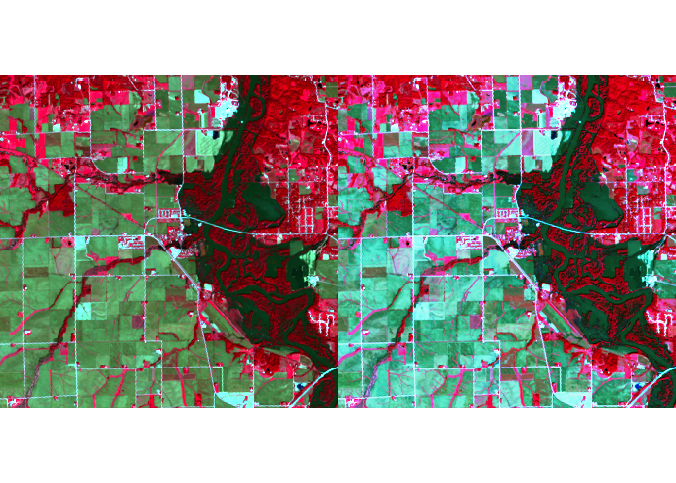
#nir-swir1-r
par(mfrow = c(1,2))
plotRGB(r, r = 6, g = 5, b = 4, stretch = "lin")
plotRGB(r, r = 6, g = 5, b = 4, stretch = "hist")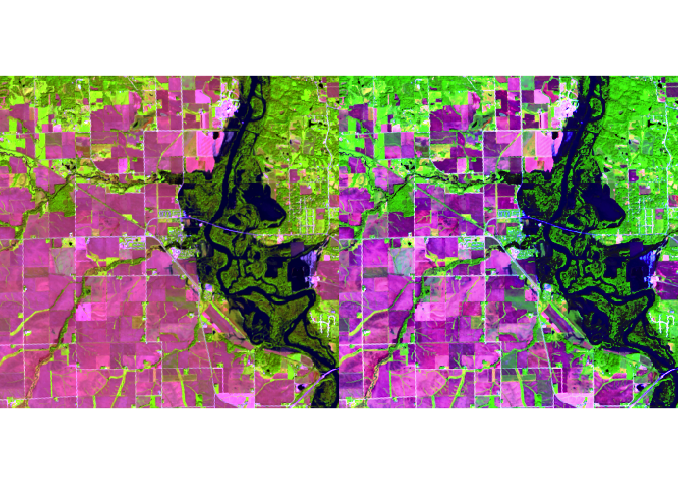
#g-nir-b,my choice
par(mfrow = c(1,2))
plotRGB(r, r = 3, g = 6, b = 2, stretch = "lin")
plotRGB(r, r = 3, g = 6, b = 2, stretch = "hist")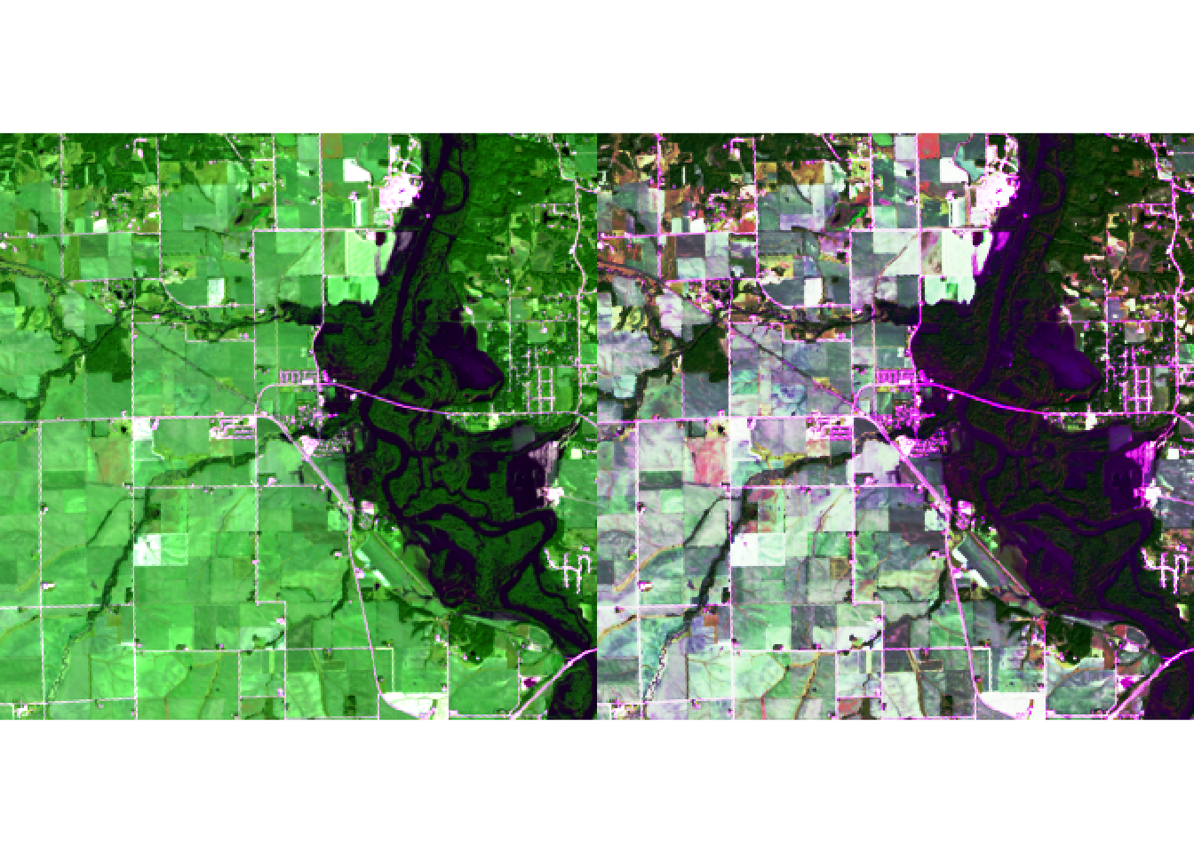 # Question 4 ### Q4.1 Local Operation
#ndvi
ndvi = (r$band5 - r$band4) / (r$band5 + r$band4)
palette1 = colorRampPalette(c("blue", "white", "red"))
plot(ndvi, col = palette1(256))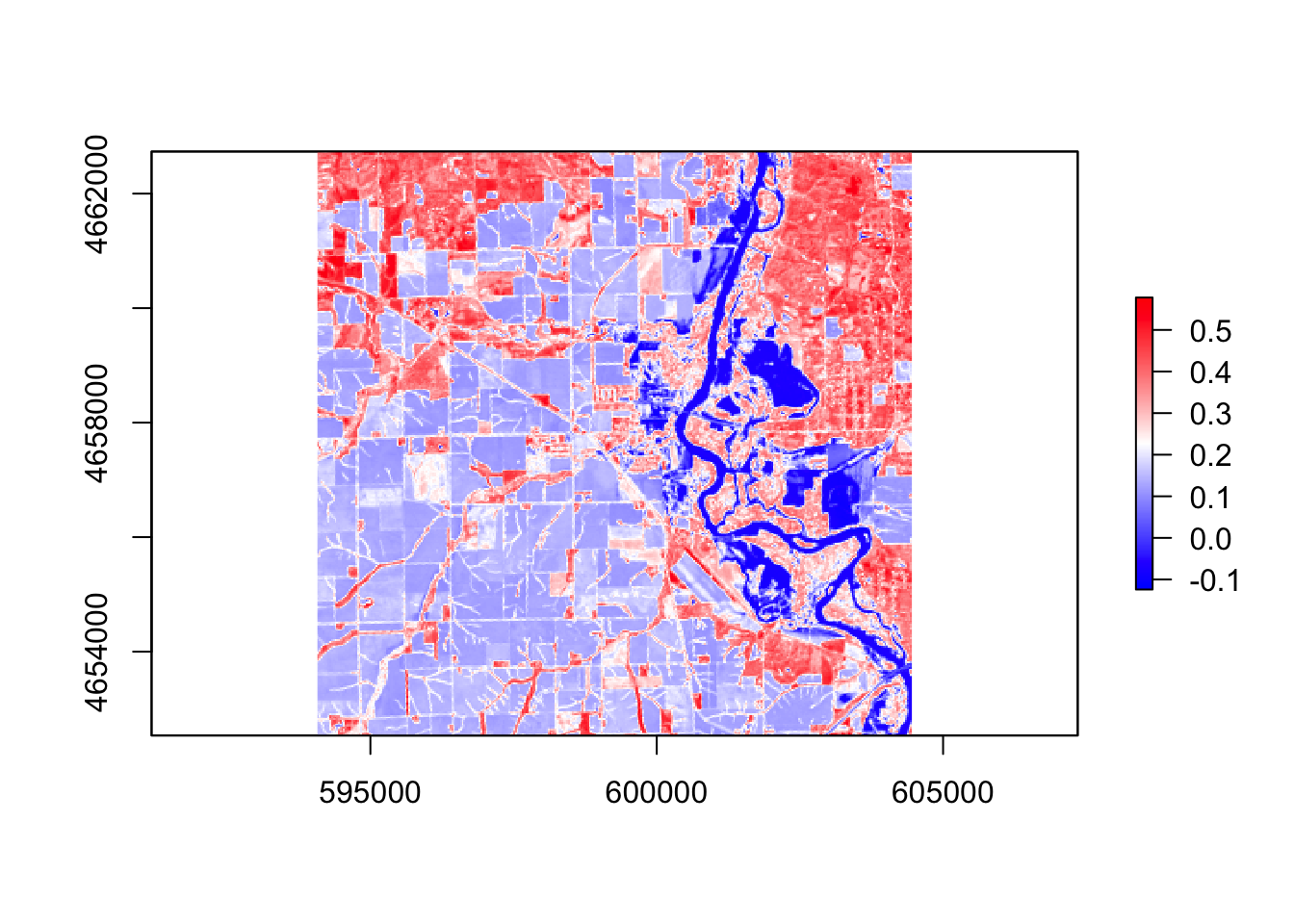
#ndwi
ndwi = (r$band3 - r$band5) / (r$band3 + r$band5)
palette2 = colorRampPalette(c("blue", "white", "red"))
plot(ndwi, col = palette2(256))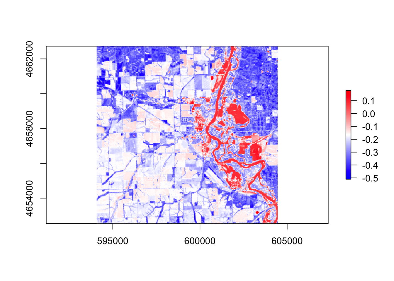
#mndvi
mndvi = (r$band3 - r$band6) / (r$band3 + r$band6)
palette3 = colorRampPalette(c("blue", "white", "red"))
plot(mndvi, col = palette3(256))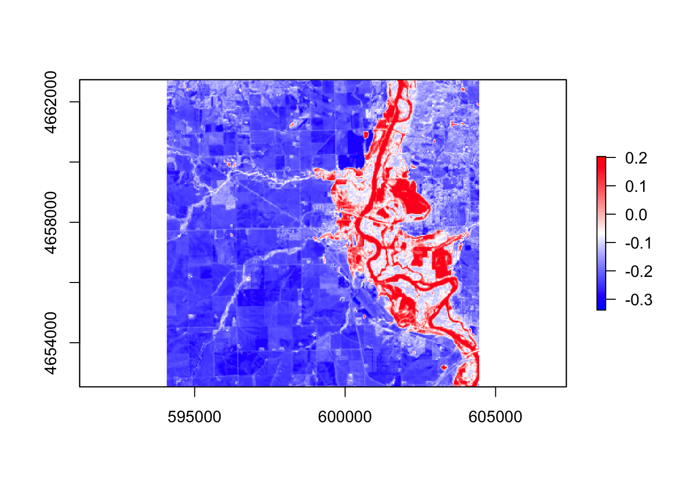
#wri
wri = (r$band3 + r$band4) / (r$band5 + r$band4)
palette4 = colorRampPalette(c("blue", "white", "red"))
plot(wri, col = palette4(256))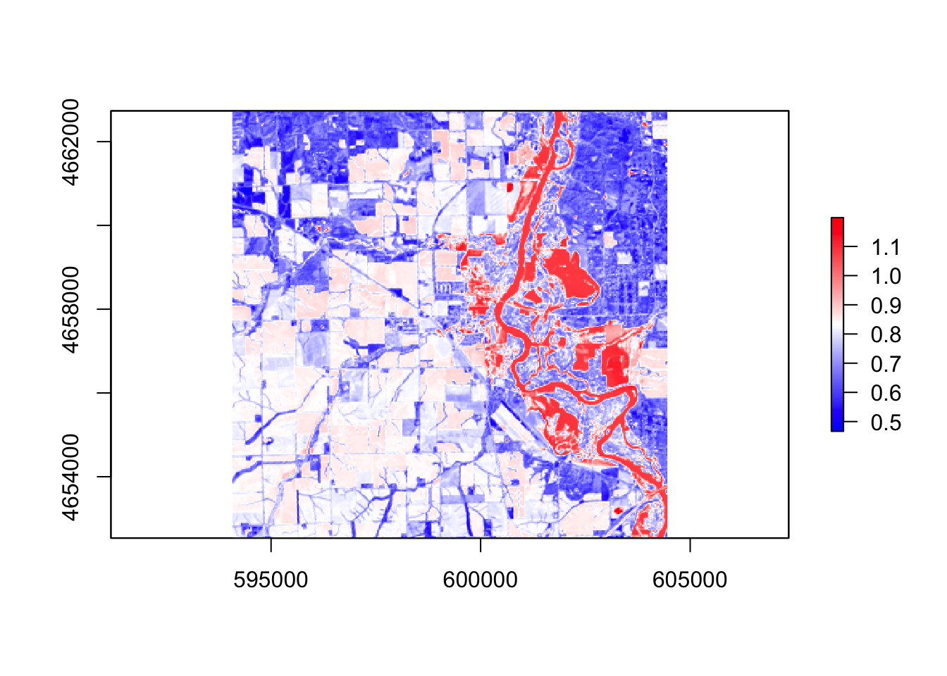
#swi
swi = 1 / sqrt(r$band2 - r$band6)
palette5 = colorRampPalette(c("blue", "white", "red"))
plot(swi, col = palette5(256))
### Q4.2 Thresholding
#ndvi
thresholdingN = function(x){ifelse(x <= 0, 1, NA)}

flood = calc(ndvi, thresholdingN)
plot(flood, col = "blue")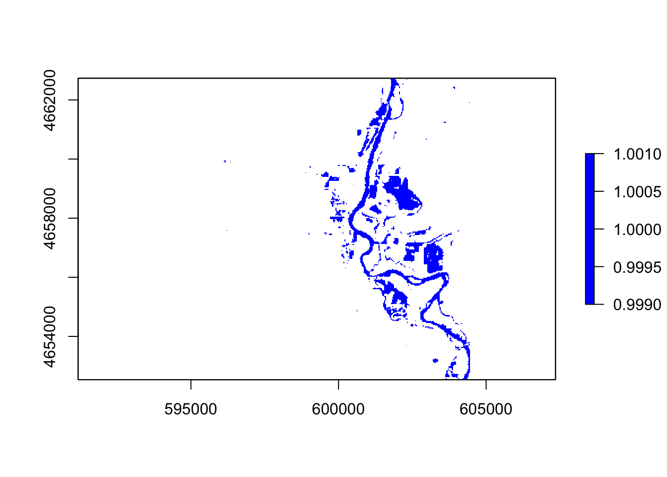
#ndwi
thresholdingD = function(x){ifelse(x >= 0, 1, NA)}

flood2 = calc(ndwi, thresholdingD)
plot(flood2, col = "blue")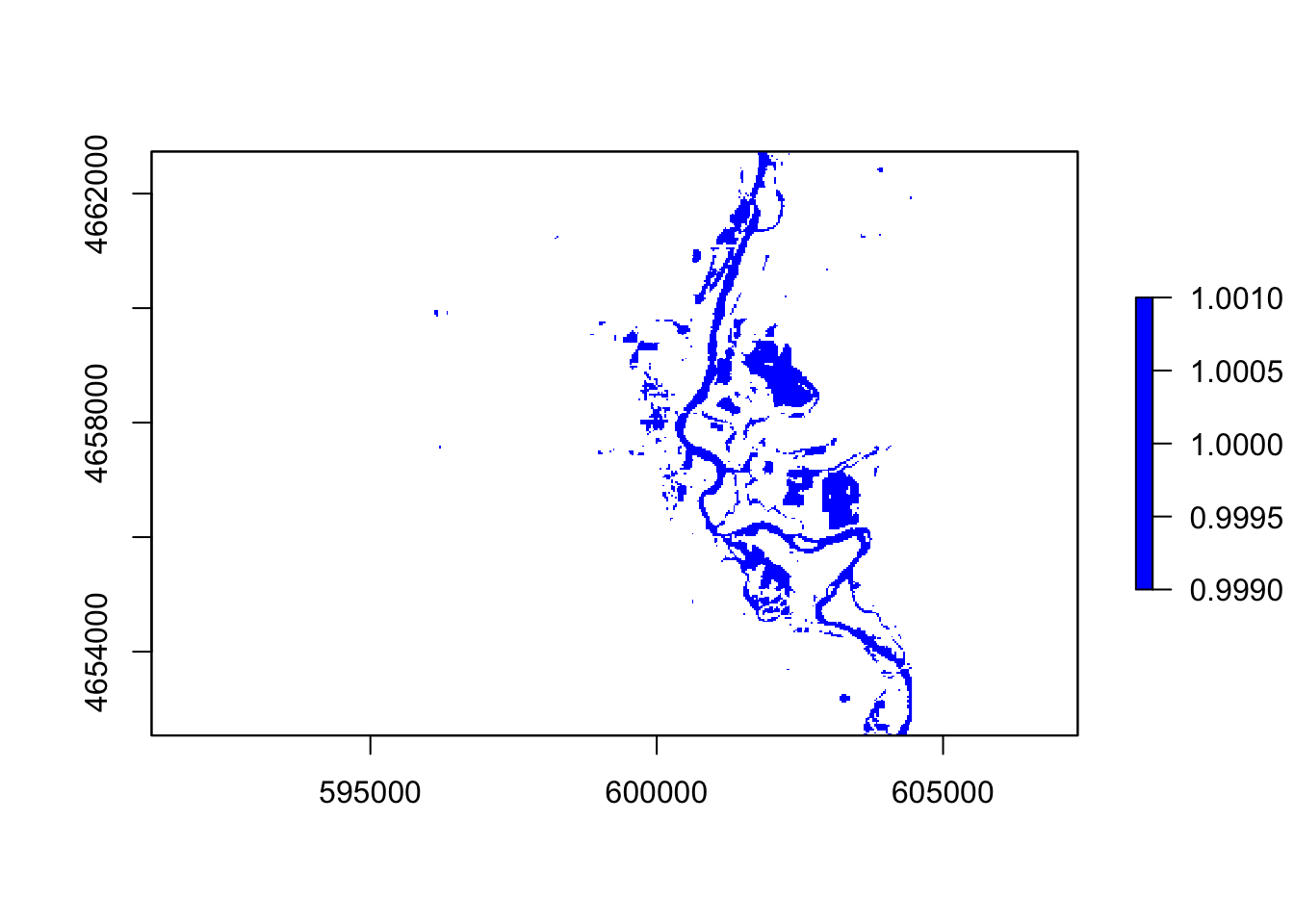
#mndvi
thresholdingM = function(x){ifelse(x >= 0, 1, NA)}

flood3 = calc(mndvi, thresholdingM)
plot(flood3, col = "blue")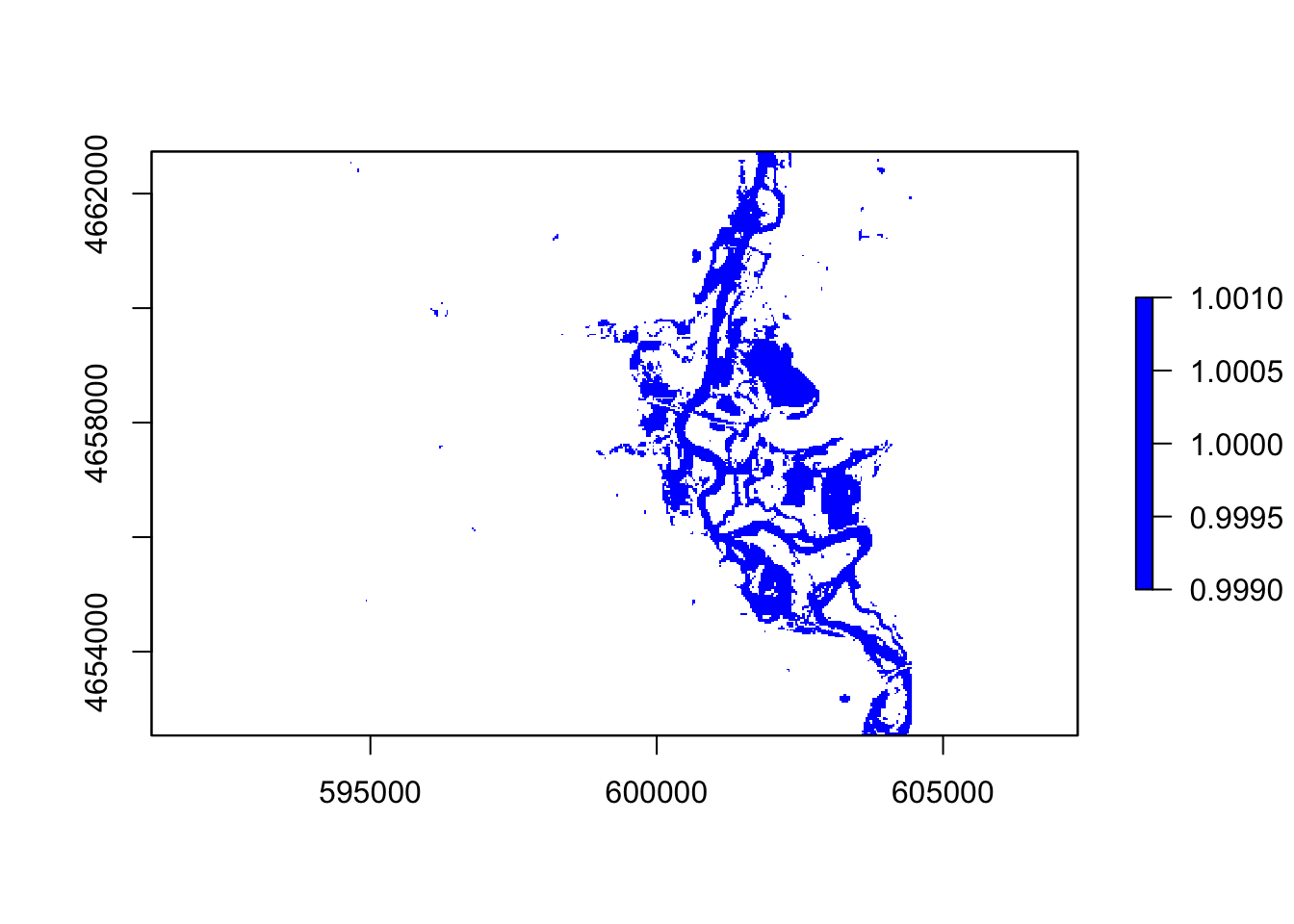
#wri
thresholdingW = function(x){ifelse(x >= 1, 1, NA)}

flood4 = calc(wri, thresholdingW)
plot(flood4, col = "blue")
#swi
thresholdingS = function(x){ifelse(x <= 5, 1, NA)}

flood5 = calc(swi, thresholdingS)
plot(flood5, col = "blue")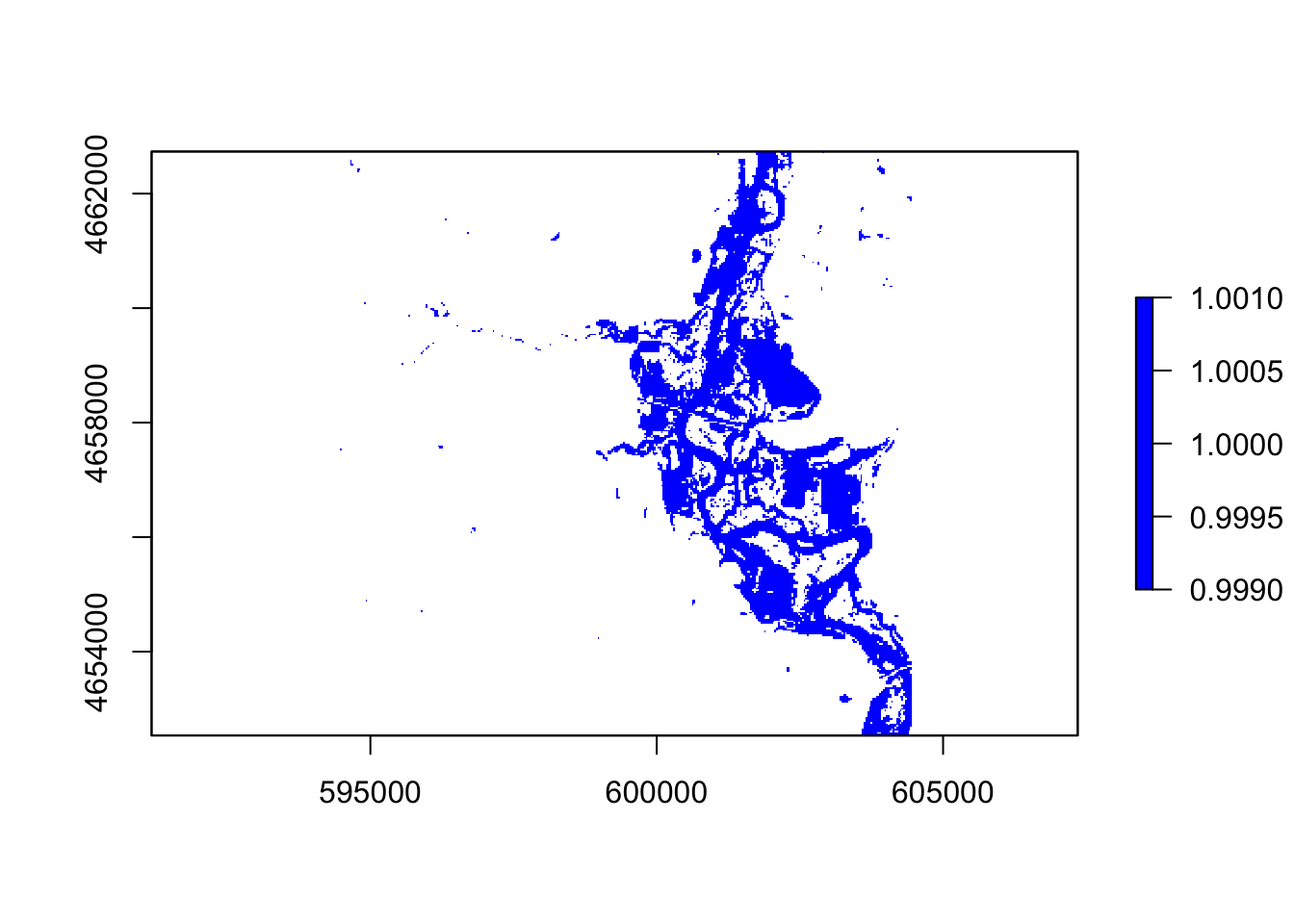
#stack
flood_stacks = stack(flood, flood2, flood3, flood4, flood5)%>%
  setNames(c("ndvi", "ndwi", "mndvi", "wri", "swi" ))
plot(flood_stacks, col ="blue")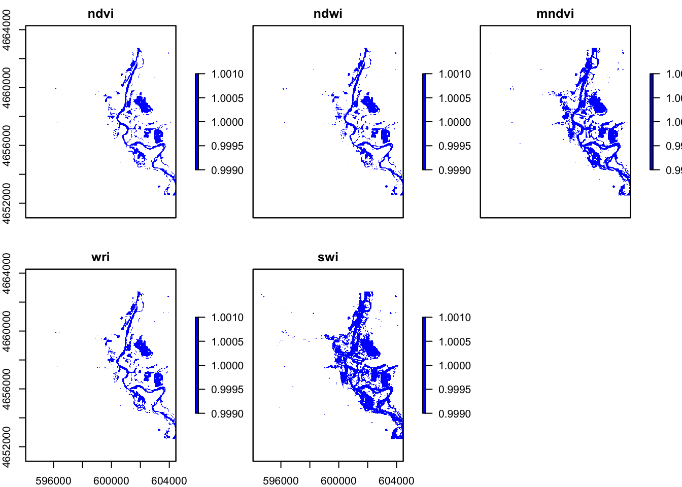
4.4 Question
In these five images, they all showing the floods around the river, However, the ndvi, ndwi, and wri look familiar compared with mndvi and swi because of the calculation and water threshold are different.
Question 5
Q5.1 set.seed
set.seed(09032020)
v = getValues(r)

idx = which(!is.na(v))
v = na.omit(v)
5.2 extract and check
k2 = kmeans(v, 12, iter.max = 100)

knew_raster = ndvi
values(knew_raster) = NA
knew_raster[idx] <- k2$cluster

plot(knew_raster, col = RColorBrewer::brewer.pal(5, "Spectral"))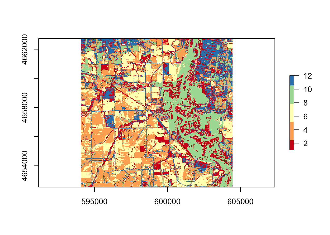
5.2 Question
The data was extract in 2 datasets and one of the datasets has 340 346 6 in the sets and the which is tolds there’s 117640 total rows and column in 6 layers.
5.3 flood category
k3 = kmeans(v, 12, iter.max = 100)
knew_raster3 = knew_raster
values(knew_raster3) = NA
knew_raster3[idx] <- k3$cluster


flood_raster_stacks = addLayer(flood_stacks, knew_raster3)
plot(flood_raster_stacks)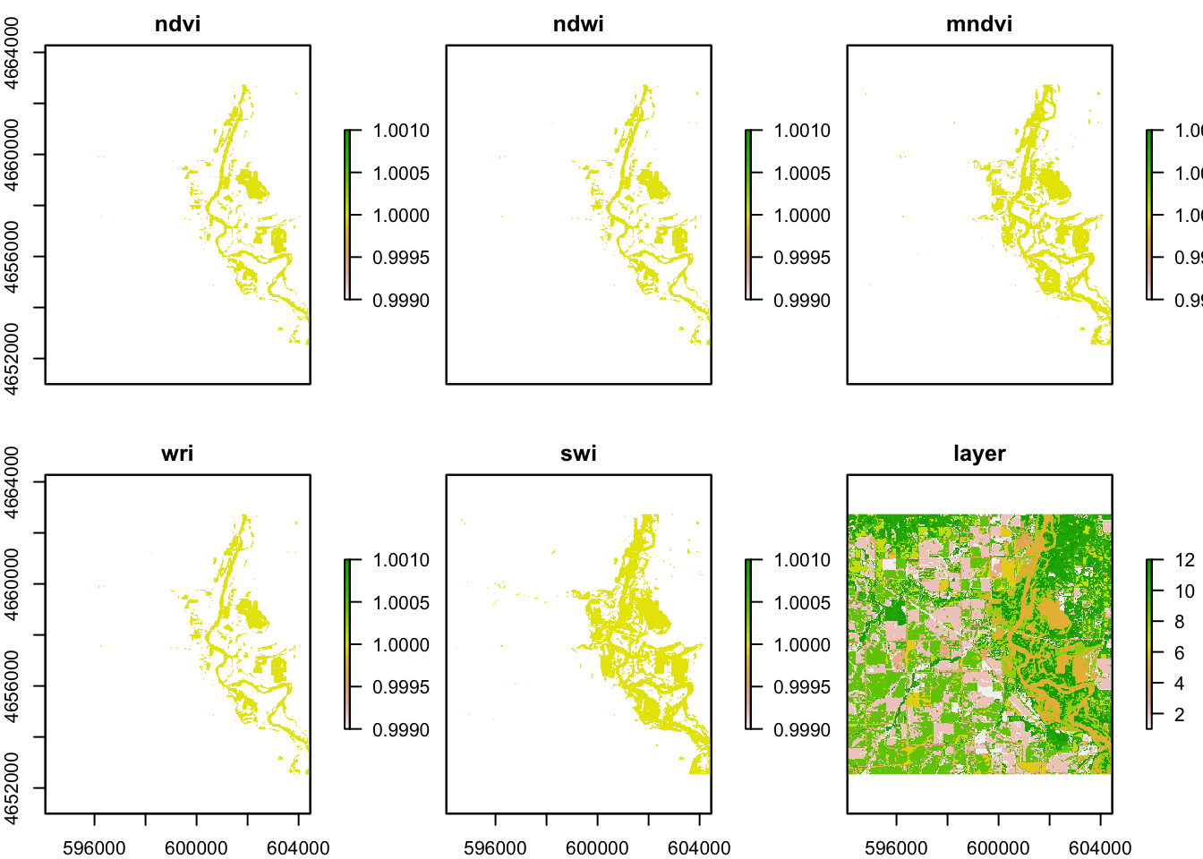
Question 6
6 Plot-Print
andvi = cellStats(flood, stat = 'sum')*900
andwi = cellStats(flood2, stat = 'sum')*900
amndvi = cellStats(flood3, stat ='sum')*900
awri = cellStats(flood4, stat = 'sum')*900
aswi = cellStats(flood5, stat = 'sum')*900
aknew3 = cellStats(knew_raster3, stat = 'sum')*900

flood_summary = bind_rows(andvi = cellStats(flood, stat = 'sum'),
andwi = cellStats(flood2, stat = 'sum'),
amndvi = cellStats(flood3, stat ='sum'),
awri = cellStats(flood4, stat = 'sum'),
aswi = cellStats(flood5, stat = 'sum'),
aknew3 = cellStats(knew_raster3, stat = 'sum'))

knitr::kable(flood_summary,
caption = "Flood Summary",
format.args = list(big.mark = ",")) %>%
kableExtra::kable_styling("basic", full_width = TRUE, font_size = 16)| andvi | andwi | amndvi | awri | aswi | aknew3 |
|---|---|---|---|---|---|
| 6,666 | 7,212 | 11,939 | 7,212 | 15,201 | 788,708 |
mapview(flood_raster_stacks, col = RColorBrewer::brewer.pal(5, "Spectral"))The reason I thinks the cell values not an even number is because the calc function has determine the visualization as using the integer number to making the resolution filling in the map and the map fill out the area with a similarity color to make the visualization more efficient.