Libraries

# SPDS
library(tidyverse)
library(sf)
library(units)
# Data
library(USAboundaries)
library(rnaturalearthdata)
library(rnaturalearth)
# Visualization
library(gghighlight)
library(ggrepel)
library(knitr)

source = "/Users/xingxin/Github/geog176a-summer-2020-lab1/"

Background

In this lab, 4 main skills are covered:

Ingesting/Building sf objects from R packages and CSVs. (Q1)
Manipulating geometries and coordinate systems (Q2)
Calculaing distances (Q2)
Building maps using ggplot (Q3)

Question 1 : Datasets

1.1 Define a Projection

eqdc = '+proj=eqdc +lat_0=40 +lon_0=-96 +lat_1=20 +lat_2=60 +x_0=0 +y_0=0 +datum=NAD83 +units=m +no_defs'

Description of this projection based on the parameters:

projection name: eqdc
Latitude of origin: 40
Longitude of origin: -96
Latitude of first standard parallel: 20
Latitude of second standard parallel: 60
False Easting: 0
False Northing: 0
Datum: NAD83
Units: m

1.2 - Get USA state boundaries

state = USAboundaries::us_states(resolution = "low") %>%
  filter(!state_name %in% c("Puerto Rico", "Alaska", "Hawaii")) %>%
  st_transform(eqdc)

1.3 - Get country boundaries for Mexico, the United States of America, and Canada

country = rnaturalearth::countries110
country_sf = st_as_sf(country) %>%
  filter(admin %in% c("United States of America", "Mexico", "Canada")) %>%
  st_transform(eqdc)

1.4 - Get city locations from the CSV file

city = read_csv(paste(source,"uscities.csv",sep = "")) %>%
  select(city, state_name, county_name, population, lat, lng)
city_sf = st_as_sf(city, coords = c("lng", "lat"), crs = 4326) %>%
  filter(!state_name %in% c("Puerto Rico", "Alaska", "Hawaii")) 
city_eqdc = st_transform(city_sf, eqdc)

Question 2 : Distance Calculation of each USA City

2.1 - Distance to USA Border (coastline or national) (km)

Five Cities Farthest from US Border
City	State	Distance to US Border
Dresden	Kansas	1012.317 [km]
Herndon	Kansas	1007.750 [km]
Hill City	Kansas	1005.147 [km]
Atwood	Kansas	1004.734 [km]
Jennings	Kansas	1003.646 [km]

2.2 - Distance to States (km)

# The distance of each city to the nearest state boundary
city_eqdc = city_eqdc %>%
  mutate(dist_state = st_distance(city_eqdc, usa_c_ml)) %>%
  mutate(dist_state = units::set_units(dist_state, "km"))

# Five Cities to US State
city_eqdc %>% select(city,state_name, dist_state) %>% slice_max(dist_state, n = 5) %>% 
  st_drop_geometry() %>% 
knitr::kable(caption = " Five Cities Farthest from State Border",
             col.names = c("City", "State", "Distance to State Border"))

Five Cities Farthest from State Border
City	State	Distance to State Border
Lampasas	Texas	308.9216 [km]
Bertram	Texas	302.8190 [km]
Kempner	Texas	302.5912 [km]
Harker Heights	Texas	298.8125 [km]
Florence	Texas	298.6804 [km]

2.3 - Distance to Mexico (km)

# The distance of each city to the Mexican border
city_eqdc = city_eqdc %>%
  mutate(dist_Mexico = st_distance(city_eqdc, filter(country_sf, admin == "Mexico"))) %>%
  mutate(dist_Mexico = units::set_units(dist_Mexico, "km"))

# Five Cities to Mexican
city_eqdc %>% select(city,state_name, dist_Mexico) %>% slice_max(dist_Mexico, n = 5) %>% 
  st_drop_geometry() %>% 
knitr::kable(caption = " Five Cities Farthest from Mexican Border",
             col.names = c("City", "State", "Distance to Mexican Border"))

Five Cities Farthest from Mexican Border
City	State	Distance to Mexican Border
Caribou	Maine	3250.334 [km]
Presque Isle	Maine	3234.570 [km]
Calais	Maine	3134.348 [km]
Eastport	Maine	3125.624 [km]
Old Town	Maine	3048.366 [km]

2.4 - Distance to Canada (km)

# The distance of each city to the Canadian border
city_eqdc = city_eqdc %>%
  mutate(dist_Canada = st_distance(city_eqdc, filter(country_sf, admin == "Canada"))) %>%
  mutate(dist_Canada = units::set_units(dist_Canada, "km"))

# Five Cities to Canada
city_eqdc %>% select(city,state_name, dist_Canada) %>% slice_max(dist_Canada, n = 5) %>% 
  st_drop_geometry() %>% 
knitr::kable(caption = " Five Cities Farthest from Canadian Border",
             col.names = c("City", "State", "Distance to Canadian Border"))

Five Cities Farthest from Canadian Border
City	State	Distance to Canadian Border
Guadalupe Guerra	Texas	2206.455 [km]
Sandoval	Texas	2205.641 [km]
Fronton	Texas	2204.784 [km]
Fronton Ranchettes	Texas	2202.118 [km]
Evergreen	Texas	2202.020 [km]

Question 3 : Visualizing the Data

3.1 Data

# 10 largest cities
largest_cities10 = city_eqdc %>%
  slice_max(population, n = 10)

ggplot() +
  geom_sf(data = country_sf) +
  geom_sf(data = state, lty = 3, size = .5) +
  geom_sf(data = largest_cities10, size = 1.5,color = "red") +
  ggrepel::geom_label_repel(
    data = largest_cities10,
    aes(label = city, geometry = geometry),
    stat = "sf_coordinates",
    size = 3) +
  labs(title = "10 Largest USA Cities (by population)",
       x = " ",
       y = " ") +
  ggthemes::theme_map()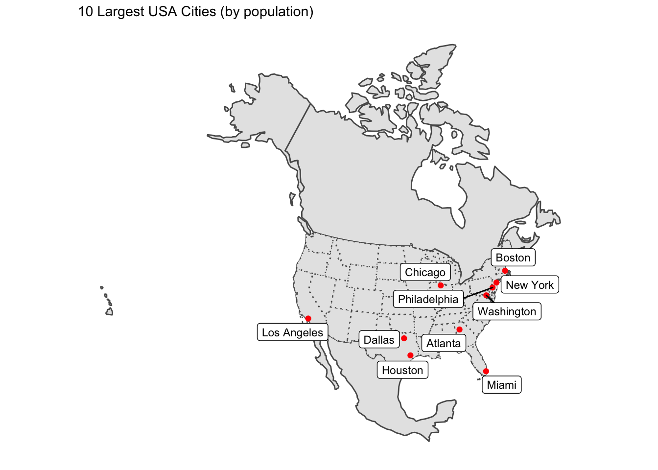

3.2 City Distance from the Border

# 5 farthest cities
farthest_cities5 = city_eqdc %>%
  slice_max(dist_border, n = 5)

ggplot() +
  geom_sf(data = city_eqdc, aes(col= as.numeric(dist_border))) +
  scale_color_gradient(low = 'blue', high = "red", name = "Distance (km)") +
  geom_sf(data = state, size = 0.5,lty = 3, fill = "NA",) +
  geom_sf(data = farthest_cities5, size = 1, color = "black") +
  ggrepel::geom_label_repel(
    data = farthest_cities5,
    aes(label = city, geometry = geometry),
    stat = "sf_coordinates",
    size = 3) +
    labs(title = "City Distance from National Border and The Five Farthest Cities",
       x = " ",
       y = " ") + 
  ggthemes::theme_map()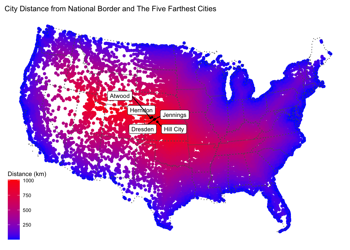

3.3 City Distance from Nearest State

farthest_cities5_state = city_eqdc %>%
  slice_max(dist_state, n = 5)

ggplot() +
  geom_sf(data = city_eqdc, aes(col= as.numeric(dist_state))) +
  scale_color_gradient(low = 'blue', high = "red", name = "Distance (km)") +
  geom_sf(data = state, size = 0.5,lty = 3, fill = "NA",) +
  geom_sf(data = farthest_cities5_state, size = 1, color = "black") +
  ggrepel::geom_label_repel(
    data = farthest_cities5_state,
    aes(label = city, geometry = geometry),
    stat = "sf_coordinates",
    size = 3) +
    labs(title = "City Distance from Nearest State Border and The Five Farthest Cities",
       x = " ",
       y = " ") + 
  ggthemes::theme_map()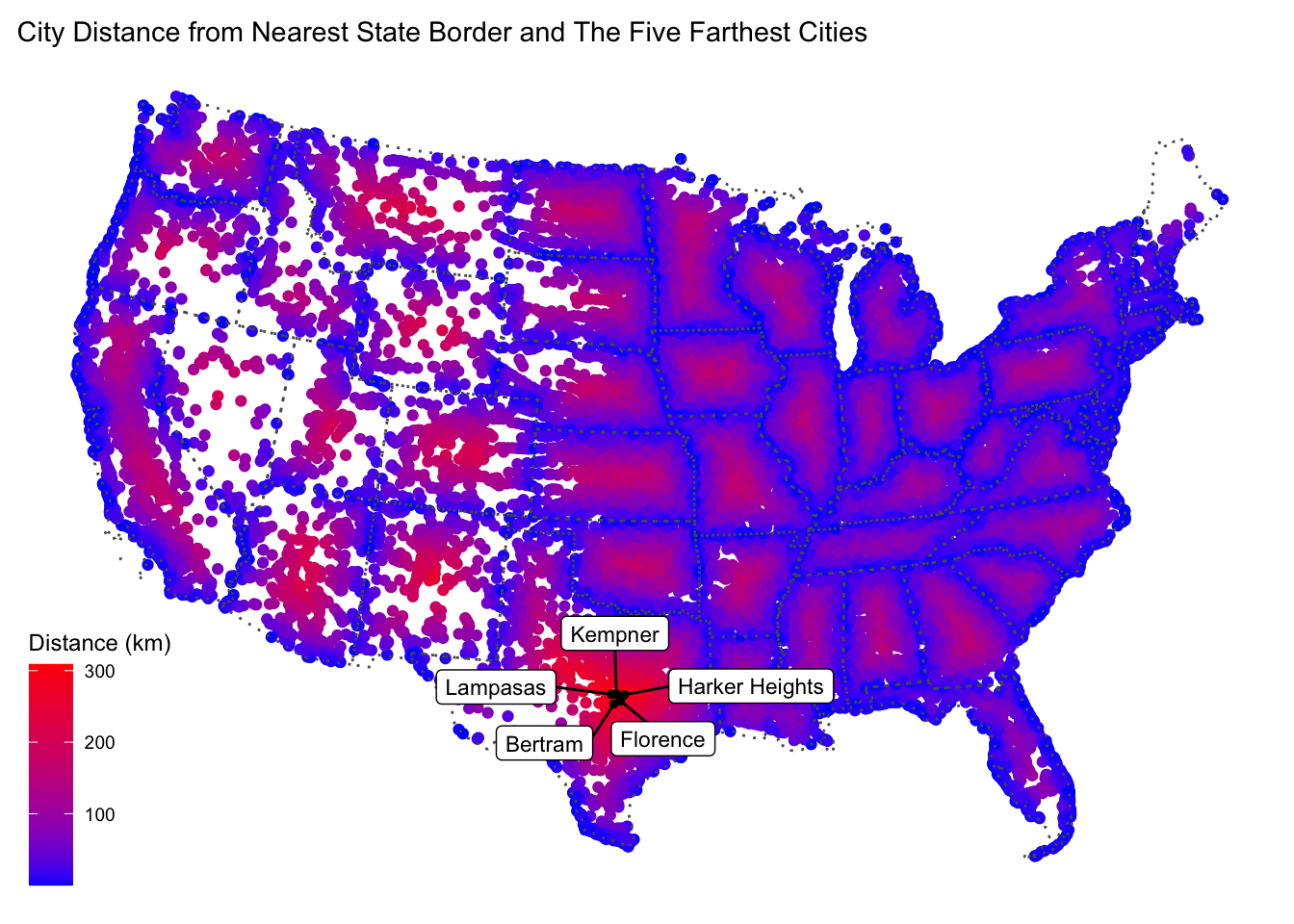

3.4 Equidistance boundary from Mexico and Canada

city_eqdc = city_eqdc %>%
  mutate(diff = abs(dist_Canada - dist_Mexico)) 
  
equal_cities3 = city_eqdc %>%
  filter(as.numeric(diff) < 100 ) %>%
  slice_max(population, n = 5)

ggplot() +
  geom_sf(data = city_eqdc, aes(col= as.numeric(diff))) +
  scale_color_gradient(low = 'grey', high = "red", name = "Distance (km)") +
  gghighlight(as.numeric(diff)<100) +
  geom_sf(data = state, size = 0.5,lty = 3, fill = "NA",) +
  geom_sf(data = equal_cities3, size = 1, color = "black") +
  ggrepel::geom_label_repel(
    data = equal_cities3,
    aes(label = city, geometry = geometry),
    stat = "sf_coordinates",
    size = 3) +
    labs(title = " Cities that are equal distance from the Canadian AND Mexican border ± 100 km",
         subtitle = "5 Most Populous Cities in This Zone",
       x = " ",
       y = " ") + 
  ggthemes::theme_map()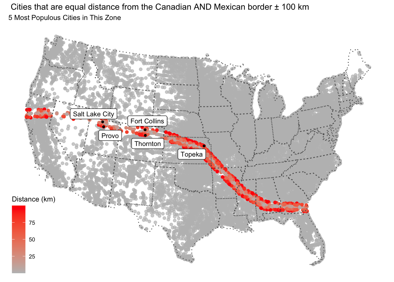

Question 4 : Real World Application

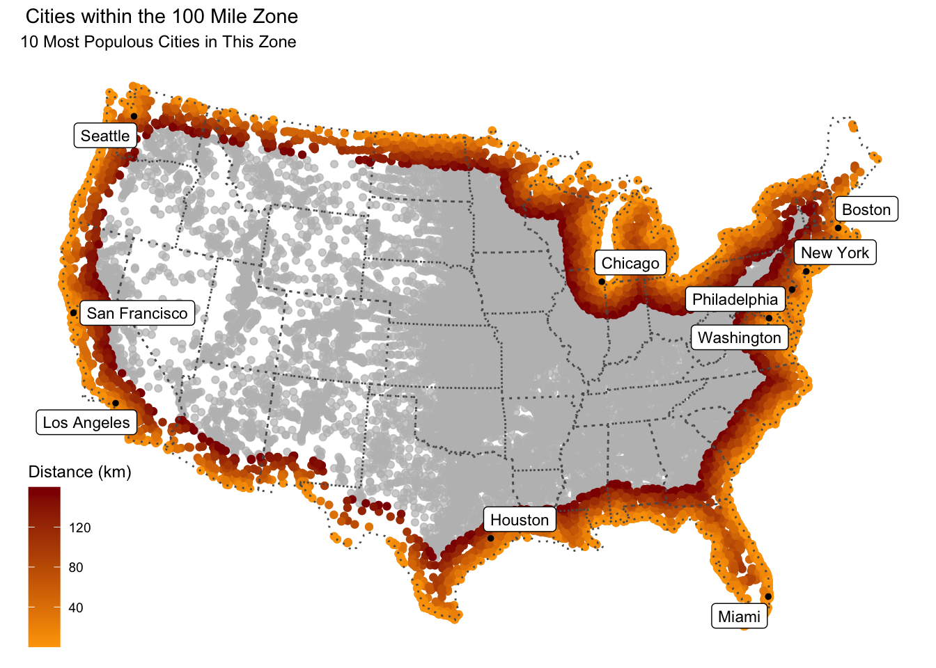
4.1 Quantifing Border Zone

# How many cities are in this 100 mile zone? (100 miles ~ 160 kilometers)

# How many people live in a city within 100 miles of the border?

# What percentage of the total population is in this zone?
zone = city_eqdc %>%
  mutate(total_pop = sum(population)) %>%
  filter(as.numeric(dist_border) <= 160) %>%
  summarise(number_cities = n(), sum_pop = sum(population), percent = 100 * (sum_pop/total_pop[1])) %>%
  st_drop_geometry() 

knitr::kable(zone,
             caption = "Cities Within 100 Miles of State Border",
             col.names = c("Number of Cities", "Number of People", "Percent of Population(%)"))

Cities Within 100 Miles of State Border
Number of Cities	Number of People	Percent of Population(%)
12283	259935815	65.43979

Does it match the ACLU estimate in the link above?

The ACLU states that “Roughly two-thirds of the United States’ population lives within the 100-mile zone—that is, within 100 miles of a U.S. land or coastal border. That’s about 200 million people.”

(1)The total number of people live in a city within 100 miles of the border calculated above is:

2.5993582^{8}

It’s about 260 million, which is higher than the ACLU’s estimation.

(2)The percent Percent of Population calculated above is:

65.4397933

which is close to the ACLU’s estimation.

4.2 Mapping Border Zone

pop_zone10 = city_eqdc %>%
  filter(as.numeric(dist_border) <= 160) %>%
  select(city, population) %>%
  slice_max(population, n = 10)

ggplot() +
  geom_sf(data = city_eqdc, aes(col= as.numeric(dist_border))) +
  scale_color_gradient(low = 'orange', high = "darkred", name = "Distance (km)") +
  gghighlight(as.numeric(city_eqdc$dist_border) <= 160) +
  geom_sf(data = state, size = 0.5,lty = 3, fill = "NA",) +
  geom_sf(data = pop_zone10, size = 1, color = "black") +
  ggrepel::geom_label_repel(
    data = pop_zone10,
    aes(label = city, geometry = geometry),
    stat = "sf_coordinates",
    size = 3) +
    labs(title = " Cities within the 100 Mile Zone",
         subtitle = "10 Most Populous Cities in This Zone",
       x = " ",
       y = " ") + 
  ggthemes::theme_map()

Lab 3

Projections, Distances, and Mapping

Xingxin Li

8/24/2020